
Abstract
Much has been written about the strengths and weaknesses of dual-Dirac as a model for jitter measurement[i]. The aim of this note is to give a gentle introduction to the topic, and how the dual-Dirac relates to practical measurements that can be made with sampling scopes and BER-based instruments.
Histograms and PDFs
A common method of viewing jitter has traditionally been to look at a sampling scope eye diagram (Figure 1.1). By setting a window around the crossing point and plotting the number of hits during a measurement, it is possible to get an idea of the movement of the data edges in time.
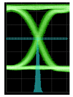
While there are issues of sampling depth with an approach such as this, it is useful as an illustration. The more samples recorded in a particular position, the more frequently the edges were in that position. This leads to the idea of the histogram being a measure of the probability of an edge falling at a particular location, or time — a Probability Density Function (PDF). The longer the sampling period, the greater the ability to represent rare events such as edges that are further away from the ideal transition timing.
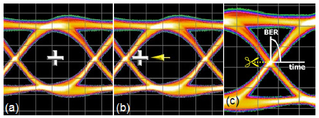
Figure 1.3 shows two example PDFs. The (a) is somewhat Gaussian, perhaps dominated by noise causing edges to move out of their ideal position. (b) is more complex. It appears that as well as some randomness in edge location,

there also seems to be two distinct peaks - two locations that occur more frequently than would be expected were the movements purely random. An example of an eye diagram that could cause such a PDF is shown in (c). There are many underlying mechanisms that could cause such a PDF; examples of impairments include Inter Symbol Interference (ISI) and crosstalk. The mechanism might also be deliberate, such as modulation on edges by a signal generator. In all cases, the mechanisms are not random, and the results are repeatable — stimulating the system in the same way produces the same result. This leads to the idea that the jitter can be divided into a random component (Random Jitter, RJ) and a deterministic component (Deterministic Jitter, DJ).
The Dual-Dirac Model in Theory
Conceptually, the dual-Dirac model of jitter is a way of taking a histogram of jitter (PDF) and making assumptions in order to divide it into random and deterministic portions. There are a number of reasons for doing this:
1) A lot of high speed digital communication standards require the total jitter (TJ) to be measured. This is the degree of eye closure due to jitter, measured at a particular BER, commonly 1x10–12. In effect this is a measure of the width of the eye crossing point, but extended downwards off the page to include even the very, very infrequently occurring events. In order to extend the distribution to include low probability events, it is important to fit actual measurements from higher-probability events to a mathematical model so lower-probability measurements can be extrapolated, as we’ll see. Ultimately, TJ is what matters for system operation, not the subcomponents.
2) An indication of whether the underlying jitter effects are random or deterministic is also very useful for R&D and troubleshooting efforts to reduce them. Some standards also suggest budgets for the RJ and DJ separately, since accumulating random effects are combined root-sumsquared and deterministic peak-to-peak values are simply summed.
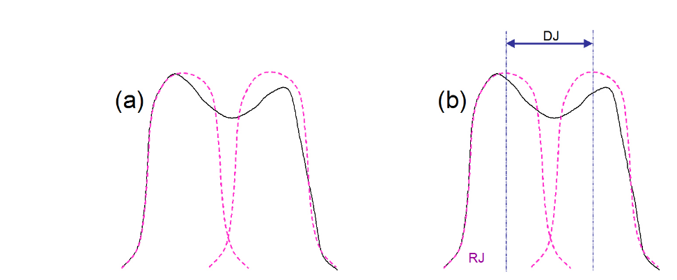
The dual-Dirac model of jitter is also called the double delta model, for reasons that will become obvious. It assumes that the tails on either side of a PDF are ultimately Gaussian in nature (Figure 2.1 (a)). It is useful to do this because Gaussians are easy to model and extrapolate down to low probabilities, and govern the randomness that is responsible for RJ. Further, it assumes that whatever DJ mechanisms are actually at work, they will be modeled purely as a separation of the two Gaussians being used to model the random effects (Figure 2.1 (b)). This is a significant assumption, but if the goal of the modeling is to produce an accurate TJ number, it is a practically useful one to make.

Using mathematical concepts, the above can be described as follows. The jitter histogram can be modeled as the convolution of a Gaussian distribution with two delta functions (Figure 2.2 (a)). It may be remembered that delta functions, or Dirac functions, are assumed to be infinitely narrow, and to have a value of zero in all locations other than at a single position where they have the value of 1. The separation of the delta functions will be assumed to represent the peak-to-peak deterministic jitter, here labeled DJ(pp).
Before going too far with this, it is worth saying that the above is a way of getting information out of a complex PDF by simplifying it — we’ll look at this in more detail later. For the moment, we are going to look at how some PDFs might look under common conditions. We will then walk through a quick reminder of how convolution works. Bringing these two sections together will then help to explain why there is some confusion about the DJ reported by dual-Dirac.
Stressed eye testing is an example of where a clean data signal is modulated with a variety of different impairment signals. Figure 2.3 shows two examples — a square wave and a sine wave.

The square wave has the closest PDF to the ideal of two delta functions (2.3 (1)). However, real signals have finite rise and fall times, and so do spend time between extremes. The sine wave case is also shown (2.3 (2)) and translated into a modulation signal of data edges in an eye (2.3 (3)). The real world deviates from the ideal, and one important effect that must be taken into account is noise, whether it appears in the amplitude or timing domains. The real PDF or scope histogram that would be measured is the convolution of the modulation PDF with the noise.
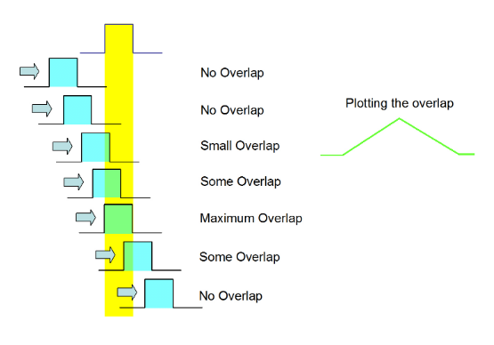
We will now run through a quick reminder of the concept of convolution. This will be far from rigorous, and more detail can be found elsewhereiv. Convolution involves taking two separate functions, moving one past the other and recording how the overlap develops. An example of two square pulses is given in Figure 2.4. Notice that the resulting function is not necessarily the same width as one of the input pulses.
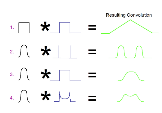
Examples (2), (3) and (4) of Figure 2.5 will be used as we build up the connection between theory and real measurements. Examples (3) and (4) are further illustrated in Figure 2.6.
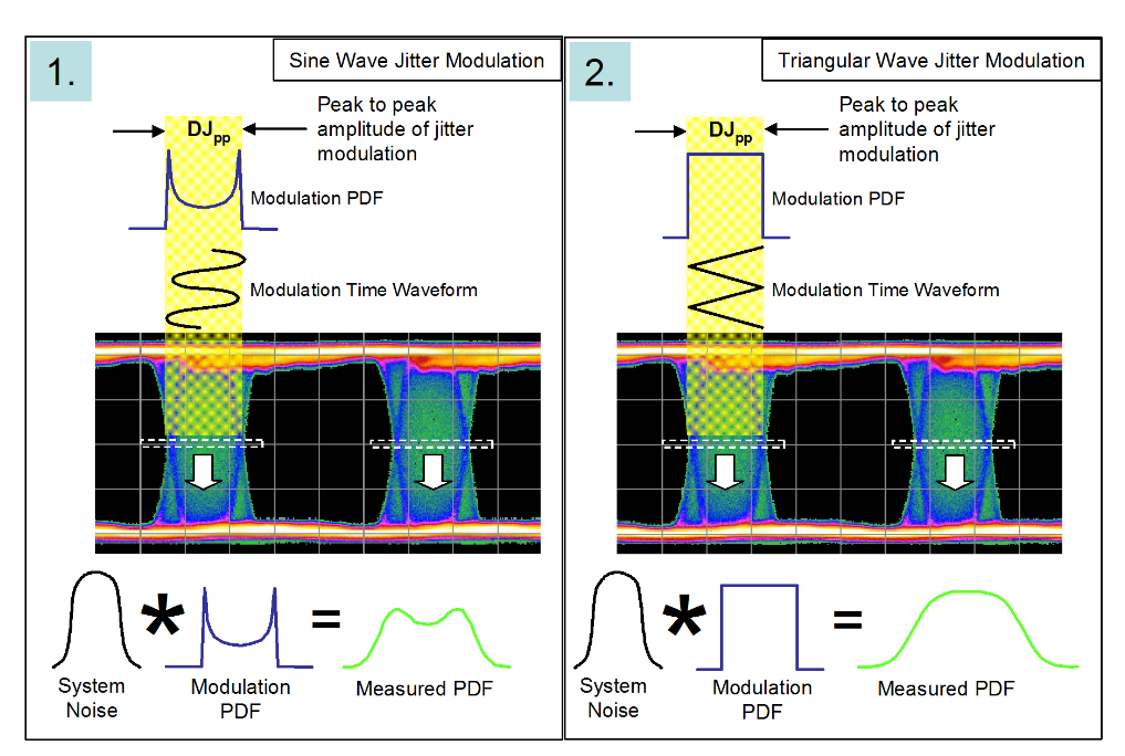
In Figure 2.6 two different modulation types are being used to cause jitter on a data eye. In the two cases the peak to peak modulation amplitudes are the same. The convolution between the idealized modulation and the system noise is shown at the bottom of the figure. The distributions are very different. We will see that although the initial modulation amplitudes are the same, once they are convolved with system noise into a histogram, and then fitted to the dualDirac model, the resulting figure for DJ(δδ) will be different to the initial modulation amplitude DJ(pp), and will be different for each example1.
The dual-Dirac model has no knowledge of the distributions that went into generating a measured PDF. The aim is to fit a Gaussian curve to each side of the measured PDF, and to designate the separation of the means to be the deterministic jitter, DJ(δδ) . It is important to realize that DJ(pp) does not equal DJ(δδ) . In fact DJ(pp) is almost irrelevant to the main job of the model, which is to get the correct eye closure due to jitter at the specified BER (TJ(10–12) ).
Let’s go back to the ideas of Figures 2.2 and 2.3, and apply them to the two example modulations of Figure 2.6. Figure 2.7 shows a sequence of steps that lead to the fitting of the dual-Dirac to the two distributions. The convolution effect is to smear out the distributions such that when the dual-Dirac model fits Gaussians to the measured histogram, the means of the Gaussians appear in different positions than might be expected from the initial modulation amplitudes.
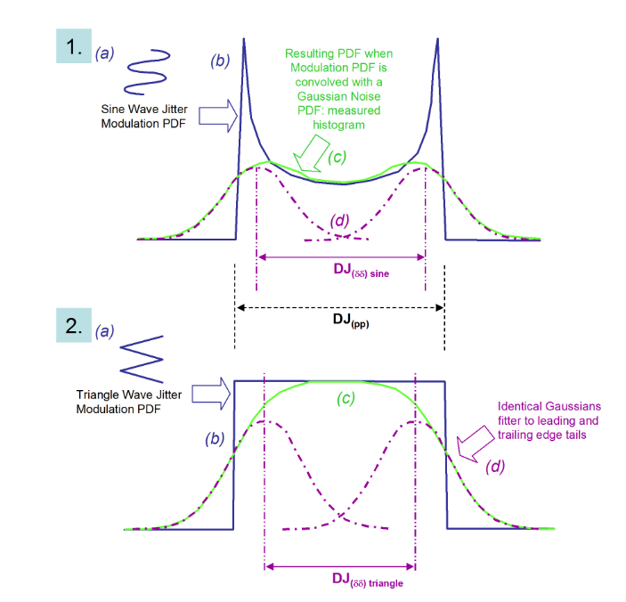
As can be seen from Figure 2.7, the idea is to fit Gaussian curves to either side of the measured PDF. The left and right extremes of the PDF should correspond to the earliest and latest arriving edges, respectively. It is intuitive that DJ pushes the earliest and latest edges apart from each other, and that noise sits on top of the earliest and latest edges, adding a random placement of the edges before and beyond where the DJ would place them. Note that the model doesn’t care what goes on in between the two tails — it just fits Gaussians to the tails and derives a separation of means.
DJ(δδ) is always smaller than DJ(pp) in practical cases. It is sometimes said that the dual-Dirac model over estimates RJ, at the expense of DJ. Some instruments measure DJ(δδ) , others DJ(pp); it is therefore important to know which DJ is being reported — most standards specify DJ(δδ) .
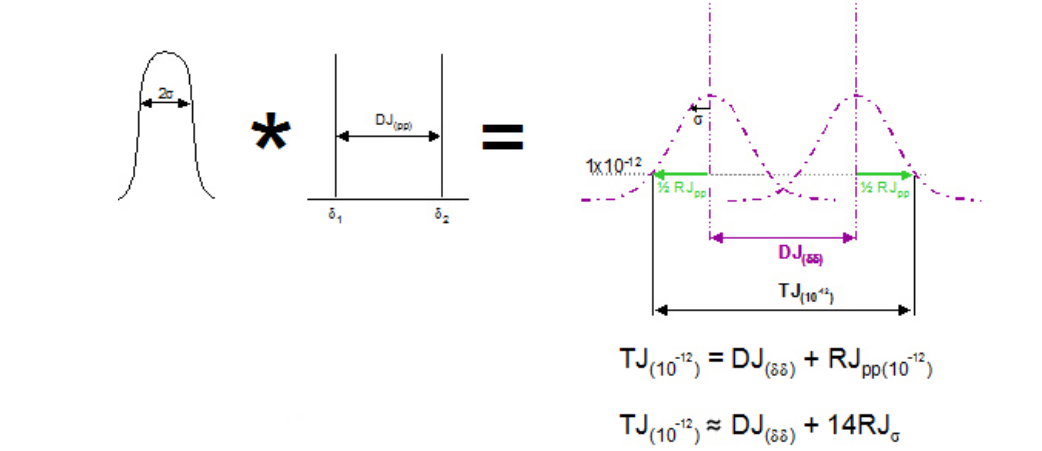
Having fit Gaussians, the math is as follows. A Gaussian is fully described by the position of its mean, its amplitude, and its width, described by its standard deviation. The math of the model assumes that the likelihood of the transition being at either peak-to-peak extreme is equal, and so the amplitude of each individual one is 0.5. Note that the model also assumes that the distributions on left and right edges are inherently identical. Notice both of these assumptions are not always true, The position of the two means give DJ(δδ) as already described. The remaining quantity is the standard deviation, which describes how fat the Gaussian is. Once fitted, this is easy to derive in theory, and also corresponds to the slope of the Gaussian.
The aim of the model is to provide TJ(10–12). This can be achieved by adding together the derived DJ(δδ) with the peak to peak RJ at the required BER level. Obviously the peak to peak width of RJ changes depending upon the depth that it is viewed at which is why it is important to use the correct value. Alternatively, the standard deviation value, RJσ, may be used. There is a well known relationship for Gaussian curves that relates BER to RJσ [v][vi].

It is from this that the commonly used approximation that to get RJ(pp)(10–12), RJσ should be multiplied by about 14. This works well providing RJσ is known accurately, but it is intuitively obvious that small errors in RJσ become significant when multiplied by 14. DJ(δδ) is defined to be constant irrespective of BER level, and because it is defined as the distance between two deltas, the lack of a multiplying factor makes error in this quantity less significant than in RJσ.
When the dual-Dirac jitter distributions of several components are combined, it is not possible to just add the TJs together linearly, and here is one of the significant values in separating RJ and DJ with the model. DJ(δδ) components may be added, with the assumption that the different values are uncorrelated:

For RJ, the values must be combined differently, using the sigma’s and RSS’d together:

Many standards provide individual budgets through a communications link for allowable amounts of each. Once the subcomponents are combined, TJ(defined BER)Total may be determined as described above.
The Dual-Dirac in Practice
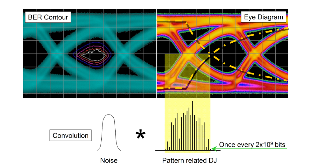
One significant problem with the practical application of the model is that the histogram taken from an eye is inherently shallow, coming from a relatively small number of samples. Many commonly used patterns are long, containing millions or billions of sequential combinations of bits. Some of the most aggressive sequential combinations of standard PRBS patterns such as PRBS-23 (223–1) and PRBS-31 (231–1) occur only once per pattern repetition. This means that although they are most likely to throw an edge the furthest (either early or late) than any other part of the pattern, this edge occurs so rarely it is highly unlikely to be picked up in an eye diagram. This is shown in Figure 3.1. In this example, the measured PDF would be the convolution of the noise with the pattern-related DJ, and obviously would be quite complex. The rarity of these deterministic effects causes them to be misinterpreted as random effects when fitting to the dual-Dirac model. The important part for the model to work is for the Gaussians to be fitted correctly to the earliest and latest edge parts of the PDF. The fit must be applied only to the tails of the distribution that are properly following the underlying Gaussian distribution, free from any residual deterministic effects.
Figure 3.2 shows how this PDF might look and how the model might be fitted to it. In (a) this distribution takes into account the earliest and latest edges even though they occur very infrequently. From this, curves may be correctly fitted and the correct TJ extrapolated. If, however, the PDF were only to be captured down to a shallower depth (as would be the case with a real eye-derived histogram) the fitting is almost guaranteed to be done incorrectly, and the wrong answers to be calculated; the rare deterministic effects would be considered as low-probability random effects. Practical ways of avoiding this will be discussed in the section on BER-based measurements.
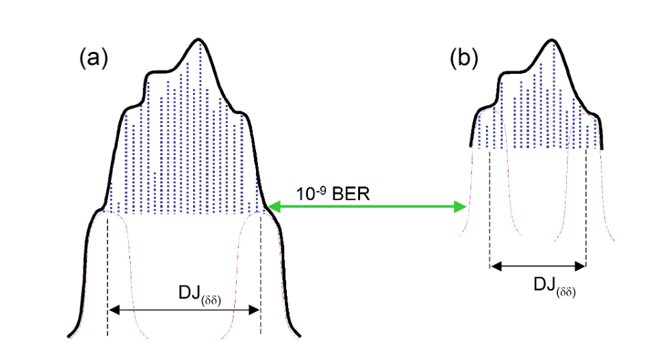
While the illustration in Figures 3.1 and 3.2 of the pattern related DJ is useful for getting the idea across, real distributions typically have so many peaks the distribution looks continuous. The DJ dominated, higher probability portions of the curve end up looking like they are following a Gaussian profile, and it becomes extremely difficult to discern where the real RJ portion begins. For a case such as this, 14 does not end up being an appropriate multiplier to relate RJσ to the peak to peak value RJpp(10–12).
A final note on pattern length and some other DJ effects: some standards such as OIF CEI[vii] are now using terminology that differentiates between the deterministic effects visible on an eye diagram (‘high probability DJ’) and those that fall below such visibility because they don’t occur frequently enough (‘low probability DJ’). DJ can derive from such things as pattern-related effects (ISI), crosstalk and power supply breakthrough (both termed PJ, or Periodic Jitter).
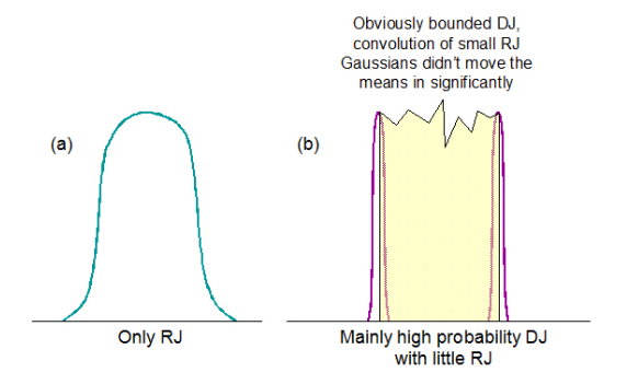
Having explored the dual-Dirac model a little above, we have seen that the more complex the DJ distribution, the more it deviates from looking like two delta functions. This has the consequence that the more the fitted means will move inward, and the smaller and more different DJ(δδ) will become relative to DJ(pp). It therefore becomes intuitive that the model is strongest at RJ/DJ separation when the signal being measured is either all RJ, or is mainly high probability DJ with little RJ to move the means inwards significantly. This is illustrated in simplistic terms in Figure 3.3.
The Dual-Dirac and BER-Based Instruments
The ideas of dual-Dirac can be translated into the BER domain also. The key point is that a BER-based instrument does not measure PDFs, but CDFs. The Cumulative Distribution Function (CDF) is related to the PDF through integration. Before giving a more intuitive explanation, it is worth having a quick reminder of how a BER-based instrument can be used to measure jitter. More details can be found elsewhere[viii][ix][x], but a brief pictorial view is given in Figure 4.1. A BER-based instrument uses a decision point to decide whether incoming data correctly compares to the expected pattern. In normal operation the decision point is placed as far as possible from the edges of the eye in order to provide the highest chance of error-free operation. However, scanning the decision point in time at the amplitude of the eye crossing point will eventually cause the decision point to collide with data edges, and for it to make incorrect decisions as a consequence (errors). Mapping the errors against time position through the eye gives a Bathtub curve, BERTScan, or Jitter Peak (all names for basically the same thing).
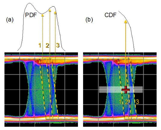
Using the idea of scanning a decision point through the crossing point, let’s look at how PDFs and CDFs differ. Figure 4.2 shows 3 example edges in an eye diagram. When measured with an eye histogram, each edge contributes to a different part of the histogram. If instead we placed a BER decision point at an arbitrary position (the red cross in the figure) and examined the effect of different edges, the result would be different. In this case, the errors recorded would be the cumulative effect of all edges that were thrown out beyond that position to the right. The further to right the decision point is moved, the fewer edges would be contributing to the recorded BER until a point might be reached where there were no edges and the BER was zero. Alternatively, moving to the left, more and more edges would be beyond the decision point and contributing errors to the BER until the BER-based instrument would lose synchronization.
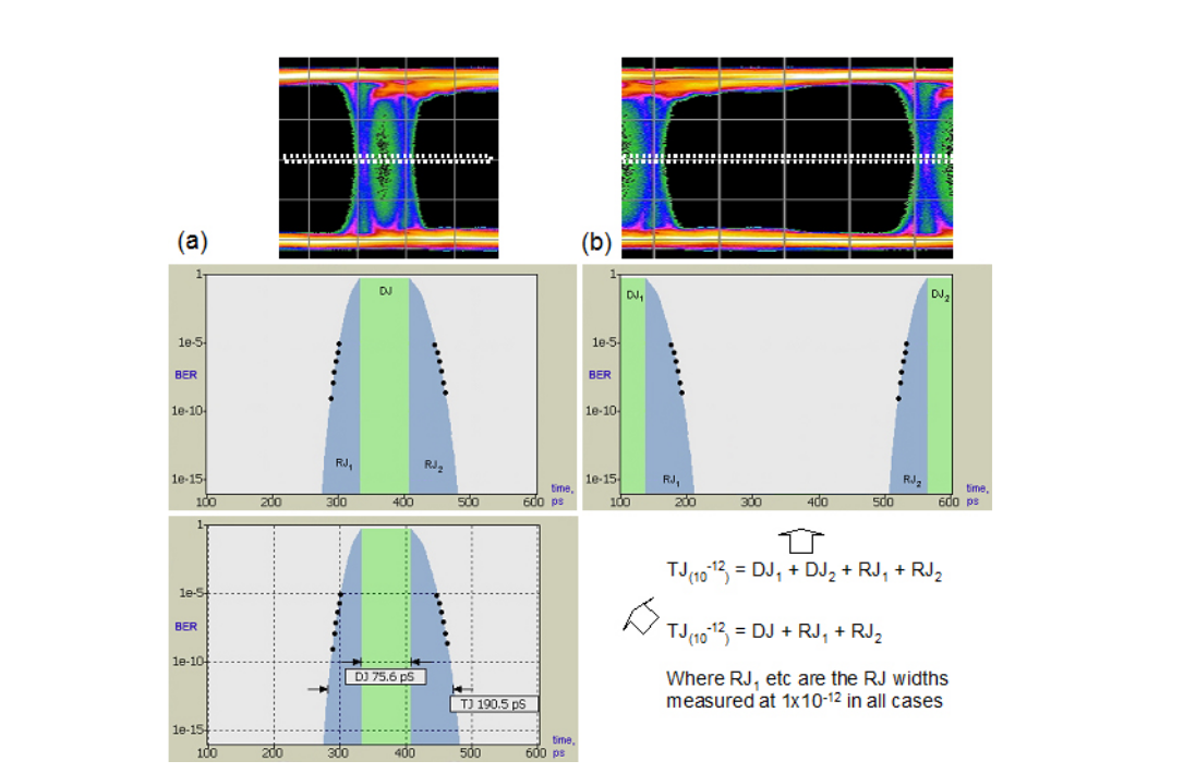
Common ways of viewing the CDF are shown in Figure 4.3, depending whether the slice is plotted through the crossing point or across the width of the eye.
TJ(10–12) , RJ(pp)(10–12) and DJ(δδ) may all be derived from the Jitter Peak. The math is different — for example, in the CDF domain, the RJ is derived by fitting a quadratic2 rather than a Gaussian when it is plotted on a log scale as it almost always is, but the end result is conceptually the same. So why measure jitter with a BER based instrument?
The first advantage of BER-based instruments is their sampling efficiency. They are capable of making a decision on every incoming bit. Where an eye histogram may only reach down to an equivalent of 10-3 or 10-4 BER, note that the Jitter Peak of Figure 4.3 has its shallowest point at 10–5, and within a few seconds is measuring 10-9. With this approach it can be practical to make a measurement that measures TJ directly — it measures the actual eye opening at a BER of 10–12. It should be noted that this requires no use of dual-Dirac related assumptions; it is the true measure of one of a system’s most important parametric aspects. However, the math is still useful for giving an idea of RJ and DJ component. For users not wishing to spend the time a true 10–12 might take, it is intuitively obvious that extrapolating down to such a level must be more accurate when it is from a large number of much deeper points than it would be on a shallow measurement such as an eye histogram.
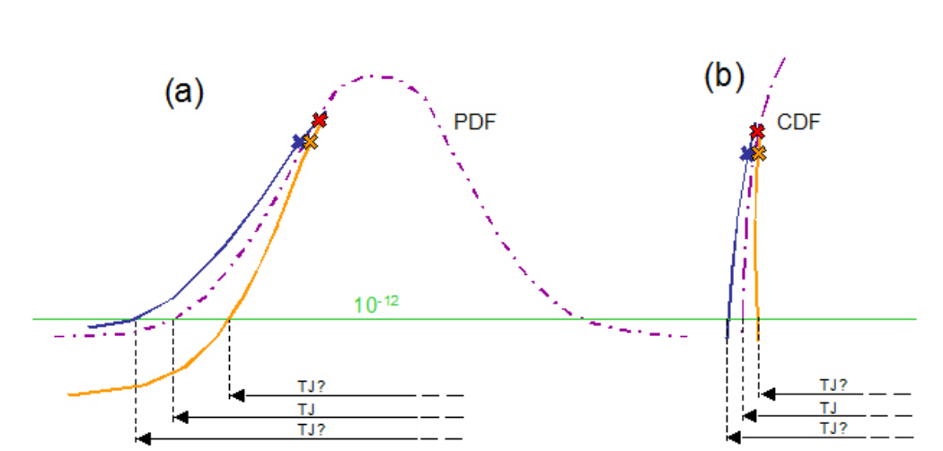
The second advantage of BER-based measurements is directly related to the first. The deep measurements made on a CDF graph prove to be much less susceptible to the effects of error. Measurement error due to noise is inevitable, but the math of the CDF curve makes it suffer less. An exaggerated example is given in Figure 4.4. The expected result is shown with the purple dashed line. The blue and orange crosses show two points affected by noise, causing a deviation from the expected curve. It can be seen that the amplifying effect of the error down at low BER levels is much greater on (a), the PDF curve, than in (b), the CDF that would be measured by the BER-based instrument. Adding this to the fact that the points being extrapolated from would be so much deeper with the BER-based measurement, it is obvious that this adds up to much improved accuracy and repeatability over an eyebased histogram measurement of jitter.
The third advantage of BER-based measurements is related to the inaccuracies that come from long patterns, as mentioned earlier. Remember that points on a Jitter Peak are acquired efficiently, and that they quickly achieve a depth of 10–9 BER. This means that a PRBS-31 with its worst case sequences appearing every 2x109 bits is much more likely to have these effects included in a measurement. However, there is a nuance here that is worth exploring, and is explained in much more detail in a very well written appendix of MJSQ[xi].

The issue is illustrated in Figure 4.5, and derives from the fact that a long PRBS such as PRBS-23 or -31 has a PDF that looks Gaussian, but is bounded — that is, although it can cause outlying edges to occur, there is zero probability of excursions beyond those that are caused by this aspect alone. This bounded behavior can cause a slope change in the PDF and CDF but for long patterns this can be a long way down (the 10–9 depth we talked about before for a PRBS-31). Ultimately we will get different end results depending upon which measured points we include in our extrapolation.
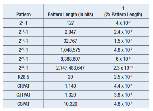
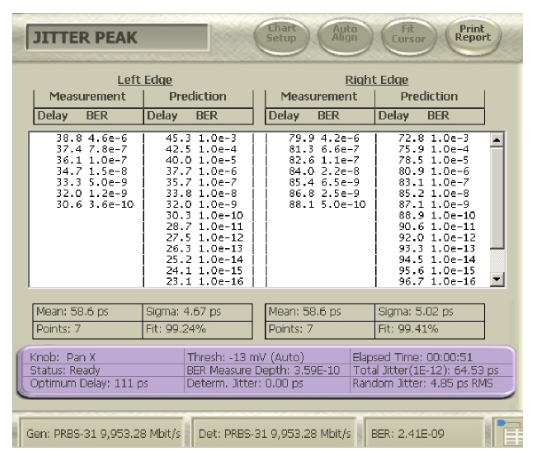
MJSQ makes recommendations about how to handle the effect of pattern length. It terms the slope change as being a ‘DJ Ceiling’, and recommends including only points in any extrapolation from below 1/(2 x Pattern Length). For example, for a PRBS-31 with approximately 2 billion bits, this would say points should only be included that were measured at a BER of 2.3 x 10⁻¹⁰ and below (See Figure 4.6). This does raise a second issue, which is that the accuracy of any extrapolation is dependent upon the number of measured points taken, as this is the best way of averaging out the effects of noise. When the first points should be below 2.3 x 10⁻¹⁰, and several measured points are required for accuracy, it can prove to be the case that waiting for points to make an accurate extrapolation to 1 x10–12 can end up involving measured points taken at 1 x 10–12, negating the need to extrapolate. Figure 4.7 shows a measured example on a BERTScope where the ‘starting BER’, or depth of the shallowest included point, is varied.
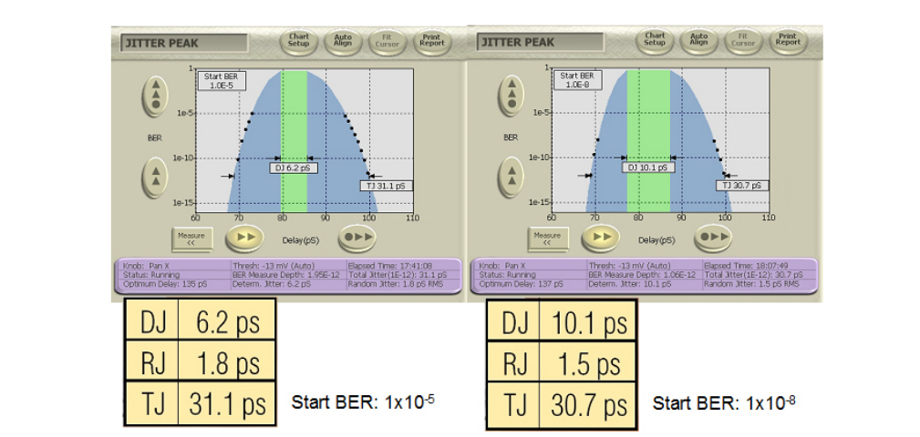
In the end, systems operate at low BER levels and it is the TJ performance that matters. The distributions that come from the dual-Dirac model can be derived from a correctly and accurately measured TJ versus BER table, as shown in Figure 4.8.
Where Did My DJ Go?
A common question when making dual-Dirac based measurements is “Where did my DJ go?” This often happens when long patterns are being used, and it is understood that DJ is present, but this is not reflected in the BERTScan or Jitter Peak result. As might be imagined given the discussion earlier on the perils of fitting Gaussian curves to distributions that are not truly Gaussian, it is very easy to fool the separation part of the model. However, as the aim of the model is to estimate the correct TJ at a given BER, the separation accuracy is not too important. An example of the effect on DJ is shown in Figure 4.7. The right hand screenshot includes less of the Gaussian-like DJ in the RJ fitting, and the reported DJ is therefore higher. Incidentally, sometimes a negative DJ can be reported by some instruments. This is typically caused by noise in the measured points throwing the curve fitting off. On the BERTScope, the DJ is always reported as zero or larger. The BERTScope gives the user control over the depth of measurements that are included in the curve fitting so that the effect of pattern length can be included.
In general, the dual-Dirac model does well separating RJ and DJ when the conditions involve RJ almost exclusively, or DJ with small amounts of RJ. For situations in between, the results are more mixed. It is important to remember, however, that TJ(at specified BER) is the main aim of the model and this is characterized well.
Summary
We’ve looked at some of the background behind the dualDirac model, and how it applies to eye histograms, and in translation to BER-based measurements. We’ve seen that it can yield good estimates of the total jitter (TJ) at the required BER level. We’ve also seen that it is important to be clear about the DJ being discussed — the model reports DJ(δδ) , the quantity used to model the correct TJ and the one specified in most standards; we’ve seen that this differs from DJ(pp), the quantity that intuitively corresponds to a known applied jitter amplitude. We have explored the effect that long patterns can have in mixing a Gaussian-like DJ distribution in with the truly Gaussian distribution that comes from RJ, and how this can affect the answer for TJ, DJ and RJ. We have also noted that true TJ values may be evaluated with a BER-based instrument without needing to use such a model, and are the most accurate measure of TJ available.

